Hello and Welcome to our final Data Visualization project. Today we will be looking at relationships between NHL siblings and their success in the league. We will see what the best group of siblings is, the most violent, and compare NHL players with siblings in the league to players without. Along the way we will see people with the exact same names as others, and explore their accomplishments in the league.
Data
The modern NHL has some dynamic sibling pairs that have found themselves in the spotlight in recent history, with the Hughes brothers and Tkachuk brothers excelling during the USA Olympic victory and for their respective NHL teams. With this in mind, we decided to look into who are the best siblings in NHL history, and look deeper at those individuals. We will also look into if NHL players with siblings are better or worse than players without siblings? Siblings often compete with one another, and push eachother to be better, so will one brother motivate others to make the NHL.
For this project there are 2 data sets. First we used skater data scraped from Hockey Reference which has a complete list of all skaters in NHL history, goalies are not included as they have a different skillset and statistical profile. This data set has 7898 rows and 24 columns, each row representing a player and their career statistics. This data set holds player information dating back to 1918 so the data set is not fully complete, with not all statistics collected for the entire history of the NHL. For instance, advanced statistics like plus minus, time on ice, or even strength goals are not collected for the early years of players. The other data set used is scraped from Wikipedia and is a list of all all siblings who have played in the NHL with an ID to determine which set of siblings each player belongs to. This data set has 711 rows and 5 columns, with each row containing 1 player from each set of siblings, along with the family name, id, and country of orgin for some players.
NHL Statistic Descriptions:
G: Goals Scored A: Assists PTS: Points = Goals + Assists PIM: Penalty Minutes pm: Plus Minus = Team Goals Scored while on ice - Goals against while on ice GP: Game Played
To combine the data sets we do a left join which keeps all of the rows from our skater data while adding columns with family name and id for players who are in the sibling data. There are a few players who have the exact same name as others, especially fathers/sons, but for our most successful sibling pairs this is not an issue. Because of how the data is stored on our skater list, we cannot look at trends with fathers/sons as I initially planned because the jr. and sr. prefixes are not included in names. This contributes to skaters with the exact same names, which raises a new question, what players with the exact same name have found the most success. For example, there are 2 players named Sebastian Aho who are not related at all, and they will be compared to all other players who have the exact same name as another player. These are some of the trends and coincidences we will explore.
`summarise()` has grouped output by 'id'. You can override using the `.groups`
argument.
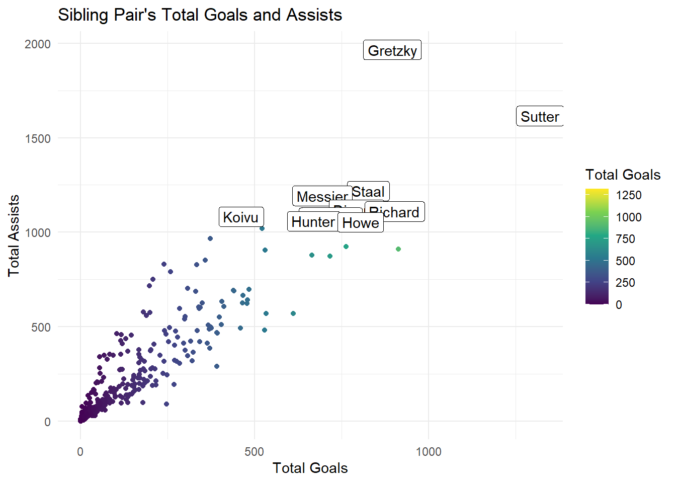
ggplot(data = g_a_sib, aes(x = tot_G, y = tot_A)) +geom_point(aes(color = tot_G)) +geom_label(data = top_ten, aes(label = family)) +scale_color_viridis_c() +theme_minimal() +labs(x ="Total Goals", y ="Total Assists",title ="Sibling Pair's Total Goals and Assists", color ="Total Goals")
This plot shows the most successful sibling pairs in NHL history in terms of goals and assists. We can see that while there are a lot of sibling pairs that have acheived impressive careers, the Sutter and Gretzky siblings clearly stand above the rest. Both of these families have impressive careers rivaling some of the best individuals in NHL history.
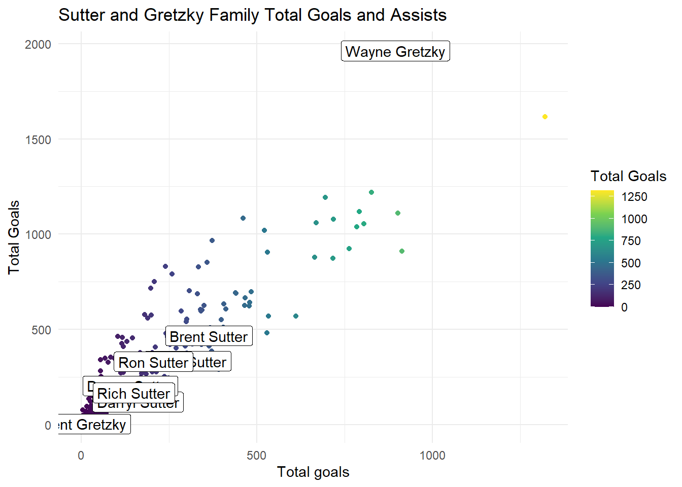
gretzky <- skaters_wsib |>filter(family =="Gretzky") |>mutate(tot_G = G, tot_A = A, tot_GP = GP, tot_PIM = PIM)sutter <- skaters_wsib |>filter(family =="Sutter") |>mutate(tot_G = G, tot_A = A, tot_GP = GP, tot_PIM = PIM)ggplot(data = g_a_sib, aes(x = tot_G, y = tot_A)) +geom_point(aes(color = tot_G)) +geom_label(data = gretzky, aes(label = player)) +geom_label(data = sutter, aes(label = player)) +scale_color_viridis_c() +theme_minimal() +labs(x ="Total goals", y ="Total Goals",title ="Sutter and Gretzky Family Total Goals and Assists",color ="Total Goals")
From this plot we can see that these two families have very different collections of careers with the Sutters putting 6 siblings in the NHL, while the Gretzky family only has 2. Many hockey fans will recognize the name Wayne Gretzky, owing to his record number of Assists and Points and nickname of “The Great One”, but less will recognize his brother Brent Gretzky in the bottom left of our plot. Brent played 13 games with in the NHL, totaling 4 PTS, while Wayne carries the pair with 2857 PTS. The Sutters have 6 siblings, all of whom played at least 400 games, and totaling immense numbers of goals and assists.
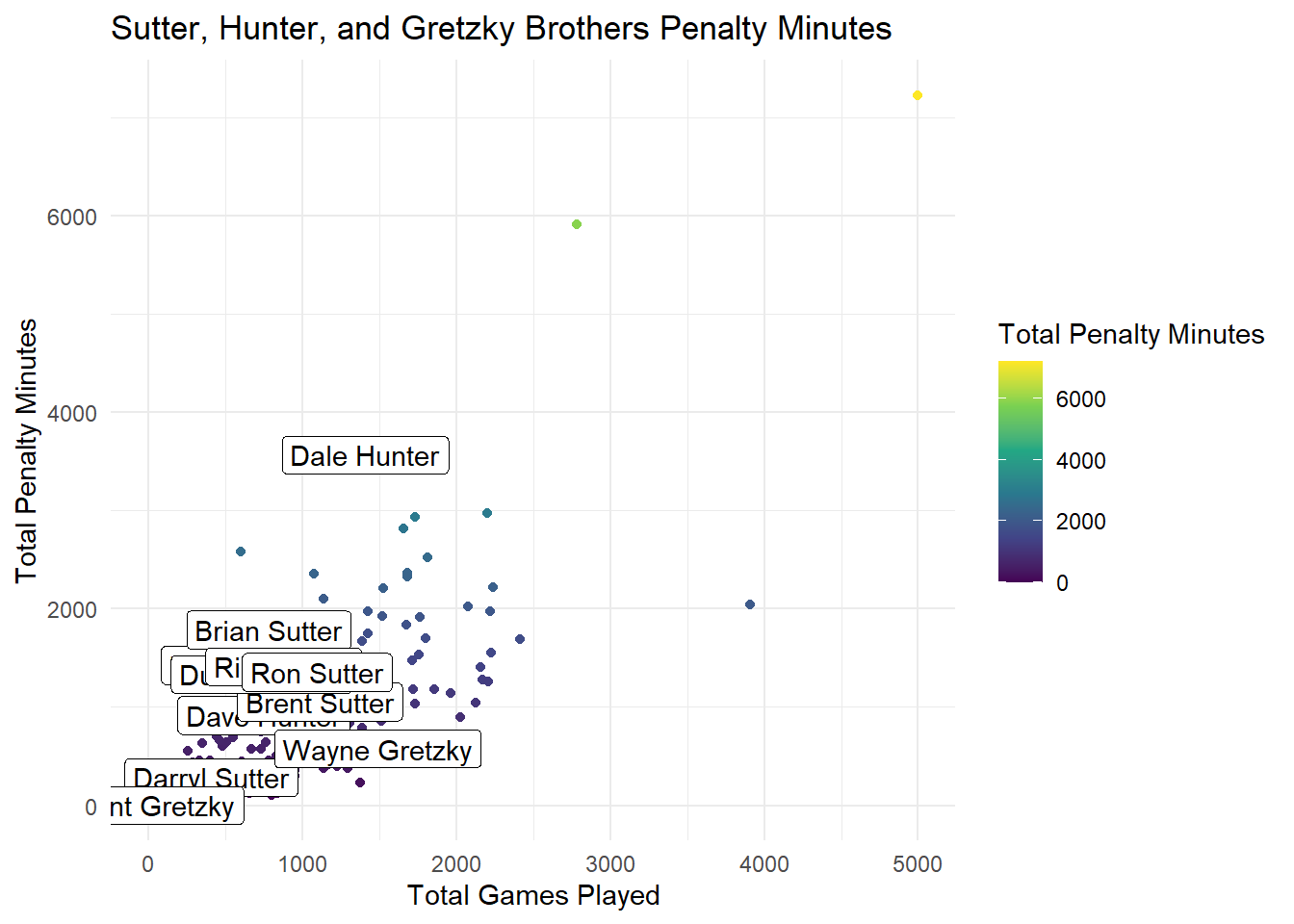
On this plot we can see that Dale Hunter’s brothers must have had a tough time growing up, with him contributing by far the most penalty minutes. The Sutter brothers also all produce a solid number of penalty minutes, and are overwhelming in their numbers, I feel for their parents who undoubtedly broke up a good amount of roughhousing. The Wayne Gretzky shows that he was more artful than violent on the ice, accumulating significantly less penalty minutes than players with the same number of games.
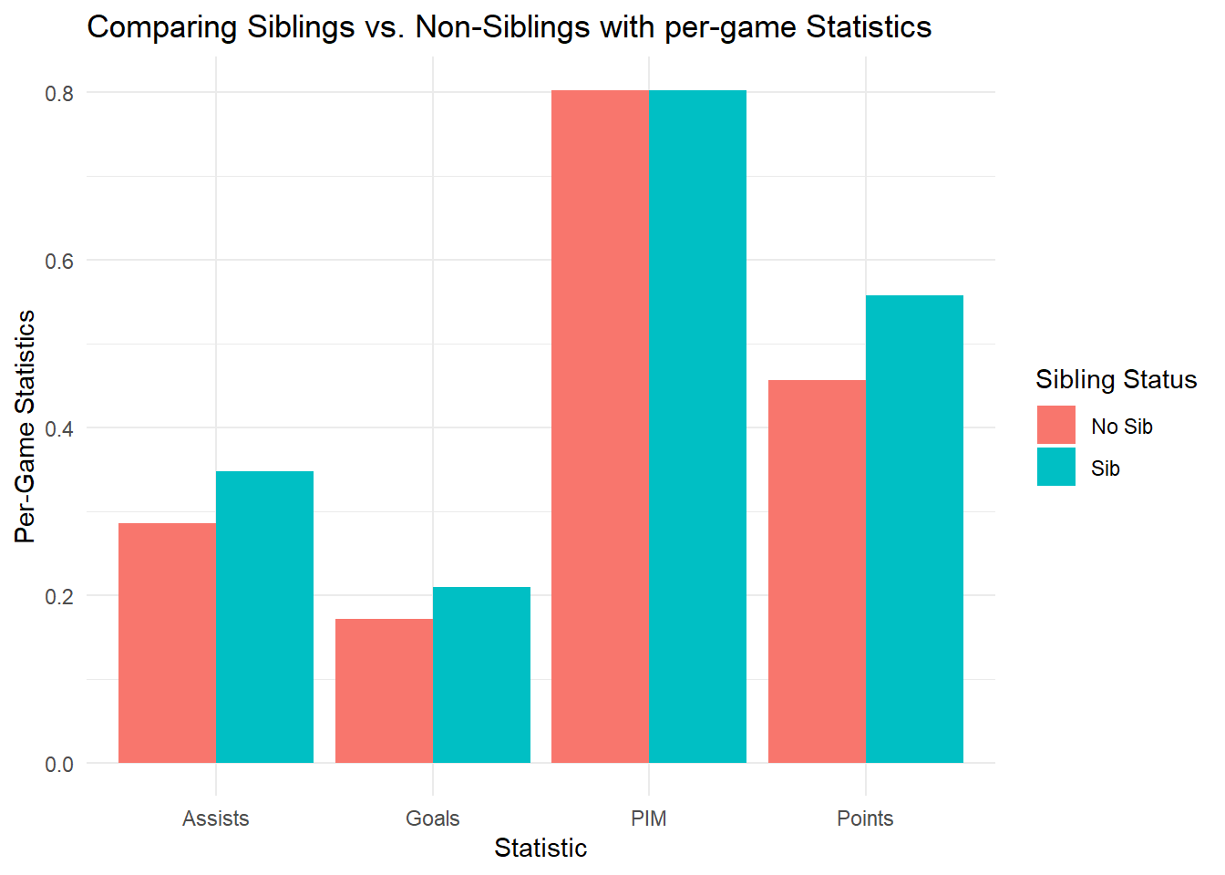
sib_comp_per_game <- skaters_wsib |>mutate(sib_ind =if_else(!is.na(id), "Sib", "No Sib")) |>group_by(sib_ind) |>filter(!is.na(PIM)) |>filter(!is.na(plus_minus)) |>summarise(Goals =sum(G)/sum(GP), Assists =sum(A)/sum(GP), Points =sum(PTS)/sum(GP),PIM =sum(PIM)/sum(GP), ) |>pivot_longer(cols =c(Goals, Assists, Points, PIM))ggplot(data = sib_comp_per_game, aes(x = name, y = value, fill = sib_ind)) +geom_col(position ="dodge") +theme_minimal() +labs(x ="Statistic", y ="Per-Game Statistics",fill ="Sibling Status",title ="Comparing Siblings vs. Non-Siblings with per-game Statistics")
This plot shows how well siblings vs. non-siblings perform per-game on average. We can see that players with NHL siblings are better in Goals, Assists, and Points per game, showing that they produce more than players without siblings in the NHL. This plot tells us that players with siblings in the NHL are better than players without NHL siblings and tend to have longer careers.
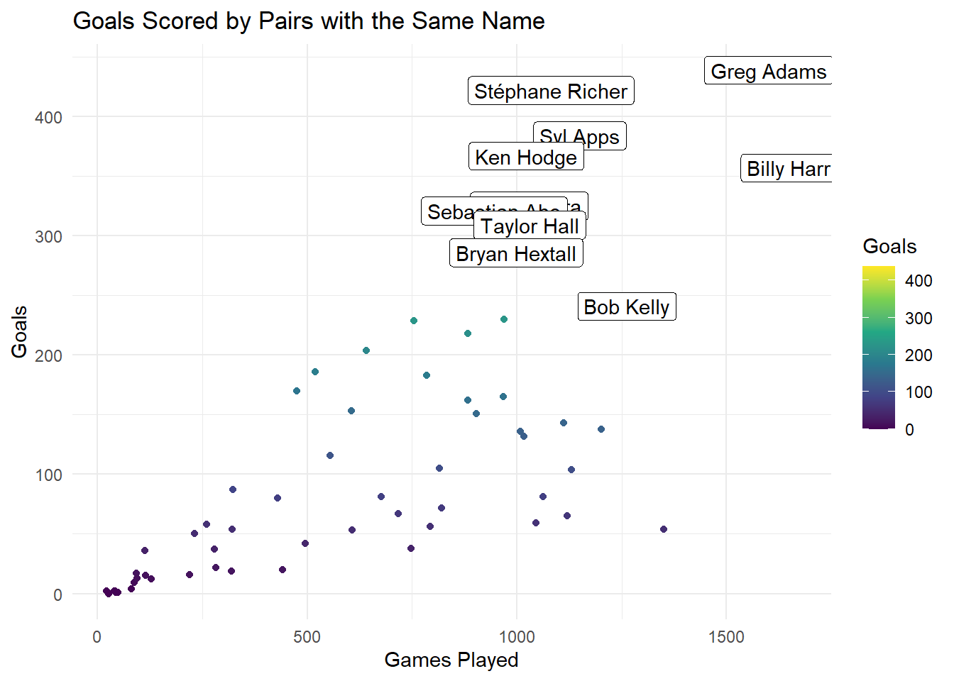
same_name <- skaters |>group_by(player) |>mutate(size =n()) |>filter(size >1) |>mutate(plus_minus =if_else(!is.na(plus_minus), plus_minus, 0, 0)) |>summarise(G =sum(G), A =sum(A), GP =sum(GP), PTS =sum(PTS), plus_minus =sum(plus_minus), PIM =sum(PIM))same_name_topg <- same_name |>arrange(desc(G)) |>slice(1:10)ggplot(data = same_name, aes(x = GP, y = G)) +geom_point(aes(color = G)) +scale_color_viridis_c() +geom_label(data = same_name_topg, aes(label = player)) +theme_minimal() +labs(x ="Games Played", y ="Goals", color ="Goals", title ="Goals Scored by Pairs with the Same Name")
This plot shows the top performing pairs of people who have the same exact name. We see players like Syl Apps Sr. and Jr., the former which was one of the greatest Centers of all time. His son would later go on to play and have a solid NHL career as well. This is contrasted with players like Sebastian Aho, with 2 players from the 2000s-2010s and coming from different countries (Sweden and Finland). The top scoring pair, Greg Adams and Greg Adams, played 10 years apart and had no relation beside the same name. It was interesting to see a number of players who had no relation with solid success in the NHL.
Conclusion
Overall, it is very interesting that NHL players with siblings tend to have more successful careers than ones without siblings. It would be interesting to see if there are studies that look into if having siblings to compete with helps your chances to make the NHL. There are some very talented sibling pairs, and it is very cool to see that some of the most talented NHL players still rise to the top. For further research it would be cool to see other familial relationships and trends around them.